Introduction to Statistical Inference & Induction

Understanding how we draw conclusions from data and its role in clinical reasoning

This page walks readers through a reading (and sometimes doing) journey. At this point I don’t attempt to house everything needed to understand statistical inference here. There are links and recommendations throughout. I’ll revisit and update, and maybe someday this will be a chapter of a book. I’m telling you all of this because I’m sitting here writing realizing that I promised I’d release this in just two days from the day I’m currently writing. I promised - I will. But it may not be done. That said - I’ll be giving you things to do throughout the page, so you’ll have to go away and come back anyway, so it should work out.

Introduction

Statistics is more than just numbers; they are a tool for understanding uncertainty and drawing conclusions about experiences based on limited observations.1 They offer a language to summarize and describe an accumulation of experience, and they provide a way to learn from our experiences (that’s where statistical inference and induction come in).

If someone tells me they have seen 500 patients with low back pain, I would love to know how many of those patients had mechanical back pain, how many had chronic back pain, how many had….. you get the point. Had that person collected information (data) from all of those experiences they could use descriptive statistics to tell me a story about the patients they have seen. Our experiences tend to be unstructured observations in an open system (the real world), as compared to research observations, which even when in an open system tend to at least try to systematically choose what information to focus on and to collect, and these days the research that gets the most attention is that which creates a closed system for us to control as much of the experience as possible to make the observation process (the experience) easier to summarize. Do you see what I’m doing here? I’m normalizing many different experiences and saying that they are ALL the same thing with different foci. They are all experiences, but on a spectrum of structure. The moment I stopped putting research and statistics into a special bin the moment they became more useful. I did this early in my career. I noticed very early that reading a research paper was like reading a reflection from someone that had made painstaking efforts to document what they could document and summarize what they observed in a language that allowed them to communicate it to me.

Let’s go back to the PT that has seen 500 patients with low back pain. If that PT documented every detail of what they did with those patients (every piece of information about every patient encounter) - then they would have a very rich story to tell. But how would they possibly tell it? To describe experiences with 500 patients is going to be much easier with the language of descriptive statistics (frequencies, means, medians, modes, standard deviations). They can even use associations between information obtained from different patients using correlations, regression (linear, simple, multiple, logistic), differences between groups of patients can be described with mean differences, standardized mean differences, and effect sizes. These are all tools that can be used to describe (summarize) this therapists experiences. The fact is that people don’t actually take the time to collect all of the information they need to use statistics to describe their experiences. It’s not because it can’t be done. It’s because it’s impractical to do. Yet despite our inability to do so, we do all agree that experience can be a good thing for our learning as clinicians. We believe, deep down, that more experience results in more knowledge, deeper understanding (we’ll come back to this soon).

So far all we’ve done is talk about statistics as a language to “describe” experiences. We have not talked about statistical inference yet. Telling me the mean age of the 500 patients with low back pain you’ve seen in the past few years is descriptive. It is not inferential until you try to tell me THE mean age of patients with low back pain. Note the difference. Telling me the mean age of the patients you’ve seen with low back pain is descriptive (and called descriptive statistics). What makes a “mean” descriptive isn’t actually that it’s a “mean.” What makes it descriptive (or any statistic for that matter) is how it’s being used. Even an “r” for a Pearson moment correlation coefficient is descriptive if what I’m doing is telling you the correlation between the age of those 500 patients and the time it took for them to walk out of the clinic “all better.” Even that is descriptive.

For example, the story might be:

I’ve seen 500 patients with LBP (n=500), the mean age was 48, and the correlation between age and the number of sessions (as a proxy for time) until they were discharged was 0.5 (r = 0.5). A regression shows that for year older a patient was, it took 3 more sessions until they were discharged, but that only accounted for 25% of the variability in the number of sessions (regression slope = 3; R^2 = 0.25).

That’s using statistics to describe a set of 500 experiences. All of that is descriptive. If that’s what the data from those experiences showed, then that’s what it showed. The math is not complicated, the math is not questionable.

In my life as a peer reviewer, associate editor, editor in chief, I’ve always found it baffling how many people confuse descriptive statistics and inferential statistics, as if they are a set of tools that are either one or the other. Well, to be fair there are some tools that are one or the other. But for the most part, the difference is what we’re doing with them, what we’re trying to say. With descriptive statistics we’re saying - this is what I observed. And as long as you didn’t make any major mathematical errors - then the descriptive statistics are not debated. They summarize what you observed (note the past tense).

Statistical Inference - Induction - Learning…..

An important book in my journey to what I think is a broader understanding of statistical inference was John Holland et al’s book: Induction: Processes of Inference, Learning, and Discovery. It’s not necessarily on statistics, and it’s very (as is everything John Holland did and wrote) interdisciplinary. And I’m not suggesting you get it or read it, just that it’s there and it certainly influenced me.

Our PT’s experience with those 500 patients becomes induction, it becomes learning, it becomes inferential statistics (statistical inference) when we start thinking about what the experience with those 500 patients tells us about people with low back pain that we have not seen but that exist (the population).

Here we are - stats 101 - the difference between a sample an a population. The sample, you’re experience. You can describe it - statistics helps you describe it. The population, the empirical domain (and that belongs with it) that exists beyond your experience but is measurable in the same way that you have measured (observed) your experience.

We describe the population with parameters. There exists a mean for all the people that exist with low back pain. There exists a correlation, a slope coefficient and an R^2 for the association between age and days of PT to meet discharge goals in the population of people with low back pain. They are all parameters. We don’t know them. We would like to know them. So, we infer them from what we have available, which data about a sample from which we can calculate statistics on the sample.

Parameters are to populations AS statistics are to samples.

Statistics can at once describe the sample (descriptive) and they can tell us something about the parameters from the population from which they are experienced (inferential).

Please note the deep philosophical statements being made here.

Learning is using what you’ve experienced to understand beyond what you’ve experienced. Sure, you must understand what you’ve experienced to learn from it - that’s what reflection is all about. Reflection is all about trying to understand what you experienced, or are experiencing (Schön,, The Reflective Practitioner).

Back to our example. If our therapist makes a claim that these numbers represent people (in this case with low back pain) beyond those people that they have seen in their experience, they are doing statistical inference:

The mean age of patients with LBP IS (not was) 48 years old, and the correlation between age and the number of sessions (as a proxy for time) until they were discharged IS (not was) 0.5 (r = 0.5). For each year older a patient IS, it TAKES 3 more sessions until they ARE discharged, and this accounts for 25% of the variability in the number of sessions (regression slope = 3; R^2 = 0.25).

Stop - think about that paragraph, compare them, what’s missing?

If you actually stopped and thought about those two paragraphs - the descriptive (about the sample) and the inferential (inferring to the population) - did you identify what is missing from the inferential paragraph?

Uncertainty and Precision

The big confusing step that takes us from descriptive statistics to inferential statistics is uncertainty and precision.

One of the first things that happens when we start doing inferential statistics is that the “statistic” that describes the sample, becomes an “estimate” of the population.

The mean is a statistic when it describes the mathematical average of the 100 die rolls that were performed. It is an estimate of the population parameter when we are doing statistical inference.

The uncertainty and precision of an estimate are provided (most often these days) by the “confidence interval.”

But to get there - we need some more preliminaries.

This list of suggested papers will close the introduction:

Stratford PW. The Added Value of Confidence Intervals. Physical Therapy. 2010;90(3):333-335. doi:10.2522/ptj.2010.90.3.333
Sim J, Reid N. Statistical Inference by Confidence Intervals: Issues of Interpretation and Utilization. Physical Therapy. 1999;79(2):187-195. doi:10.1093/ptj/79.2.186
Kamper SJ. Confidence Intervals: Linking Evidence to Practice. J Orthop Sports Phys Ther. 2019;49(10):763-764. doi:10.2519/jospt.2019.0706

Key Questions from this section for you to review:

Can you explain statistical inference?
Can you describe the difference between descriptive statistics and inferential statistics?
How does statistical inference and induction relate to learning? For that matter what does it mean to ‘learn’ based on what this introduction?
How does induction connect statistical tools to clinical reasoning?
Based on what we’ve said so far about statistical inference, how do you think this is leveraged for the process we know as “hypothesis testing”?

A deeper dive into Statistical Inference

As a recap: statistical inference is the process of drawing conclusions about a population based on sample data (come from experiences). It allows us to learn from experiences because it allows us to relate our experiences (our samples) to realities beyond our experiences (populations). That’s what it does. Later, we’ll discuss how it is then utilized in a research study to test a hypothesis (hypothesis testing).

Let’s start with a general definition confidence interval:

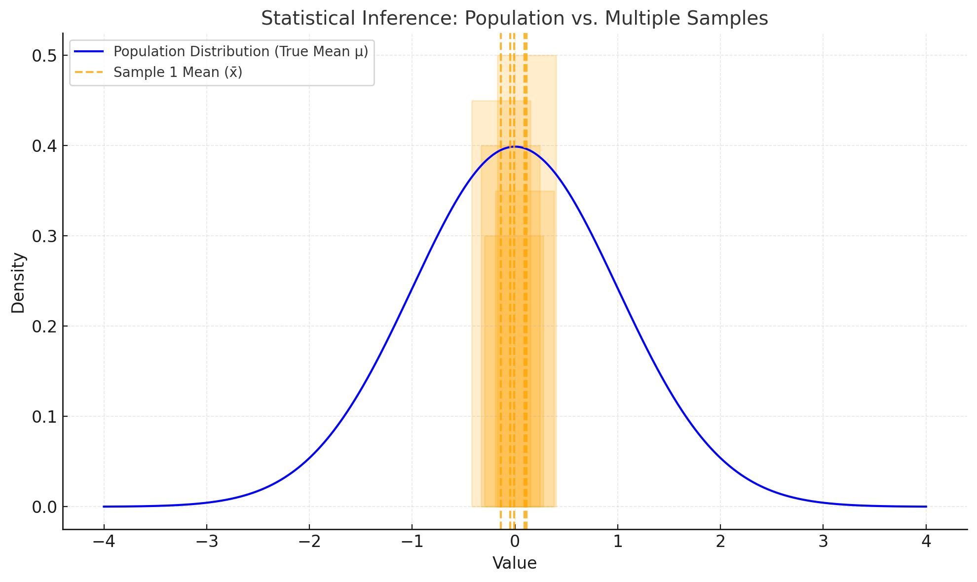
A confidence interval (CI) is a range of values, derived from sample data, that is likely to contain the true population parameter (e.g., mean) with a specified level of confidence, such as 95%. It reflects the uncertainty around the sample estimate.

There’s a tricky and argued upon aspect to CIs - likely to contain the true population parameter. It’s sometimes said that the CI is likely to contain a specified percentage of repeated sample statistic. In other words, the 95% CI is the interval that 95% of similarly collected sample statistics (by similarly collected we mean drawn from the same population using the same methods). Simulations have done a good job of demonstrating the truth of the central limit theorem, and that 95% of the repeated sample statistics are in the 95% CI, and that the the true population parameter occurs in the 95% CI, about 95% of the time. Go ahead. Read it again. The only reason I sort of understand it is because I first learned it in 1995 when I first took “Introduction to Epidemiology & Biostatistics” and I’ve been thinking about it since then - - and I only sort of understand it. What I learned over the years is to not be ashamed by that, because the best anyone can hope for is to sort of understand it. It’s not overly complicated, it’s not that its too hard to understand. It’s that there’s something about simulated confirmation that leads one to hold some doubt about whether it actually works.

Here’s what CIs ARE NOT - they ARE NOT an estimate of where 95% of future subjects (people, observations) will occur.

The 95% confidence interval estimates the range that 95% of other sample means will fall, and where we are believe (with 95% confidence) the population mean (a parameter) is (even though we have not observed everyone in the population). If a we know what the mean and standard deviation of a population are, then in theory, we have a basis of predicting what future observations drawn from that population will be (future tense).

To do so it relies on the normal distribution and two values, the standard deviation and the standard error.

Standard Deviation (sd)

The standard deviation measures the amount of variability or spread in a set of data values. It quantifies how much individual data points differ from the mean. It is a statistical calculated on samples (sd), but if based on a population, it is a parameter of the population, in which case it is abbreviated as the Greek symbol sigma ($\sigma$). (Here I’m hoping that Substack will eventually adopt the convention of inline LaTeX formatting using the markup symbols $ $ - - we can only hope.)

Formula (not inline LaTeX, but its the first step of LaTeX code integration in Substack :)

$SD = \sqrt{\frac{\sum (x_i - \bar{x})^2}{n}} $

Sorry there’s only so much wonky LaTeX formatting I can do with Substack’s inability to do inline LaTeX formatting for math equations, I’m hoping you can figure out how the below inline LaTeX code relates to the above equation:

x_i : Each individual data point
\bar{x} : The mean of the dataset
n : The number of data points

The Standard Deviation describes variability. It is useful with normal distributions. It can be a statistic (sd from a sample), or a parameter (\sigma of a population). A larger sd indicates more spread-out data; a smaller SD indicates data points are closer to the mean. We need the sd in order to calculate the SE…

Standard Error (SE)

The standard error measures the variability of a sample statistic (e.g., the sample mean) from different samples taken from the same population. It reflects the precision of the sample mean as an estimate of the population mean. To rephrase this to relate to our more general formulation of statistical inference related to experience: SE measures the variability of summarized experiences from different summaries of experiences with the same population.

Formula:

$SE = \frac{sd}{\sqrt{n}}$

Where:

sd : Standard deviation of the sample
n : Sample size

SE describes how much sample means are expected to vary if we repeatedly sample from the population. It should be intuitive that - and the equation clearly shows that - as the sample size ( n ) increases, the SE decreases, meaning larger samples provide more precise estimates of the population mean. We need the SE to calculate the CI…

For our PT example from above, as the PTs experience with patients with LBP increases in size (in theory) that PT develops a more precise understanding of patients with LBP. I say in theory because the fallibility of memory, combined with the unstructured observations, combined with bias and fallacies in thinking, there are numerous road blocks to the actuality of more experiences developing an unbiased understanding of a population.

An intuition you need to develop - for normal distributions and for sd (when thinking about a sample) and for SE ( when thinking about sample means) is well known to most anyone that has taken a stats class - and these days I think even many middle or high school math or science courses.

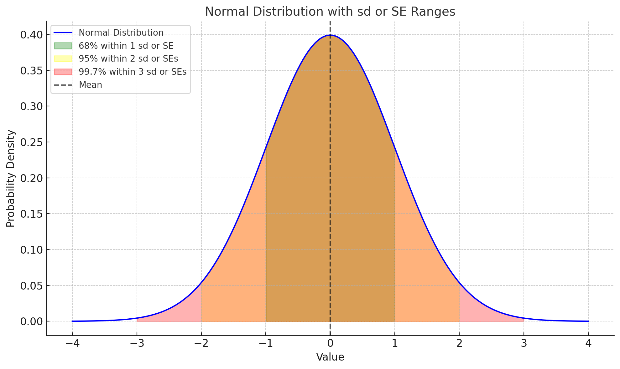
Technically +/- 1.96 sd or SE is 95%; but we often round up to 2 (which is probably closer to 96%)

Note that this same distribution can be for a sample (when using sd), or for a bunch of sample estimates (means, or other characteristics of a bunch of samples) when using the SE.

Powerful stuff for learning - not just for reading research papers. Power stuff to understand as you go through life and reflect on your experiences and attempt to learn and grow.

Confidence Interval

Here we are, back at the confidence interval, but now equipped to give your theoretical understanding of statistical inference some actualities through calculation.

The 95% confidence interval (95% CI) is a range of values derived from a sample that is likely to contain the true population parameter (e.g., mean) with 95% confidence. It reflects the uncertainty in the sample estimate due to random sampling variability by harnessing the SE and the normal properties of the normal distribution.

Formula:

For a population mean, the confidence interval is calculated as:

$\bar{x} \pm Z^* \cdot SE$

Where:

\bar{x} : Sample mean (or any other estimate)
Z^* : Z-score corresponding to the desired confidence level (1.96 for 95%)
SE = Standard error (based on sample mean)
n : Sample size
SD : Standard deviation of the sample

A population distribution with several samples drawn, sample means (which are means of samples) calculated (dotted lines), and 95% CIs for each sample generated (shaded areas). As you can see - they overlap greatly and most of them include the population parameter (mean).

Explore

At this point I think you should explore a bit on your own to develop an intuition for these concepts. But first I’d like to direct you to some older peripatetic PT posts on statistical inference that were written while I was doing activities in class on the topic.

A story of statistical inference - off the podium volume 1

Alea iacta est - off the podium volume 2

These two posts give additional insights into stats inf, but also help prepare you to do some explorations on your own.

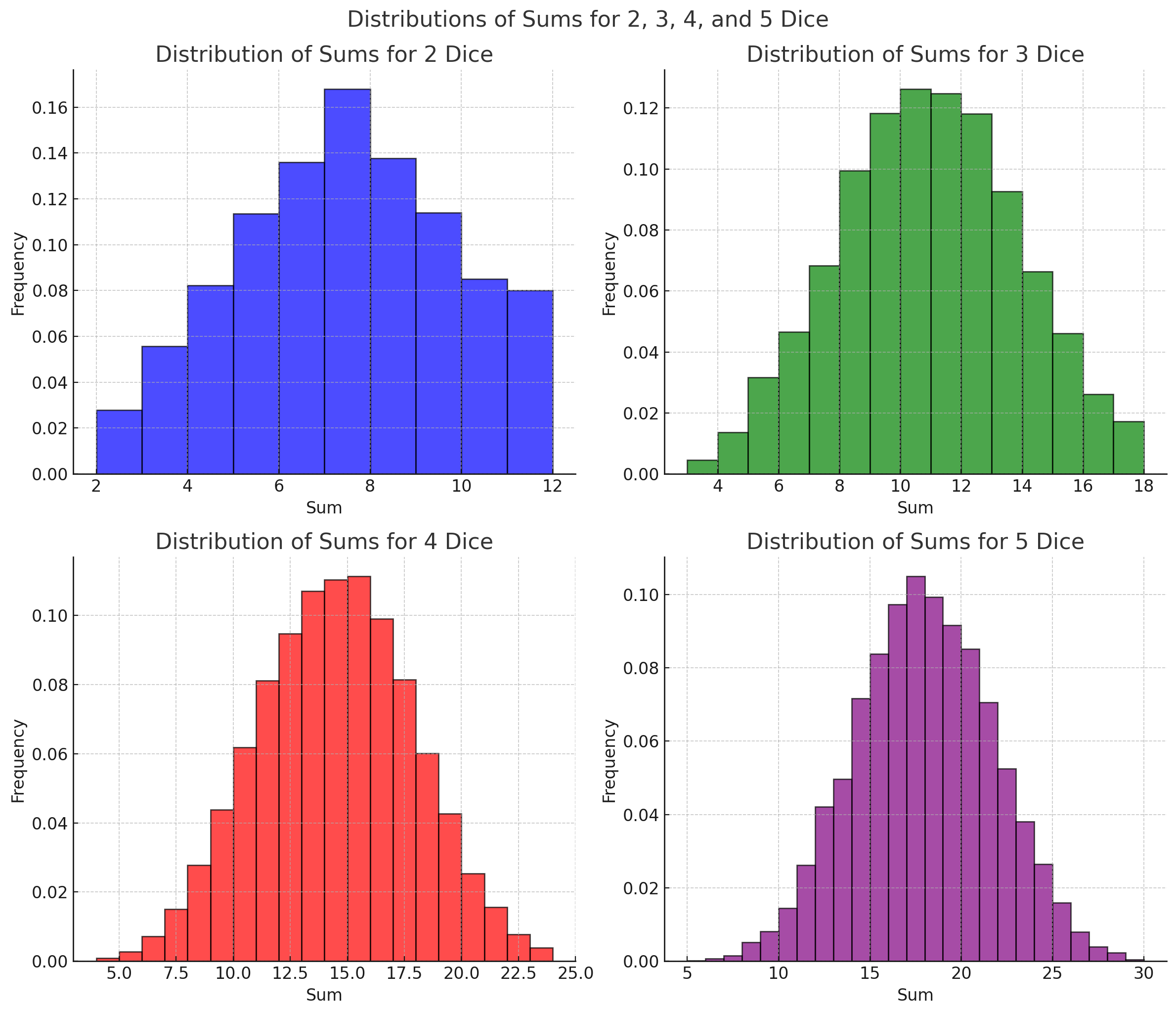
I’d like you to explore with a hands on exercise - using dice preferably since if you have at least 2 and take the sum of each roll, you’ve got a system that has a normal distribution. As you can see here - the more dice you roll, the more normal the distribution gets (“more normal” as a distribution as in smooth and symmetrical).

To explore these concepts, try this hands-on exercise using dice:

Draw Samples: Roll 2 dice 50 times and record the sums. Treat each sum as one observation, and a sample of independent sums as a sample. Your population is the infinite set of rolling 2 fair dice.
Divide Into Samples: Create smaller samples by grouping rolls into independent subsets. For example:
- One sample of 10 rolls (observations)
- One sample of 15 rolls (observations)
- One sample of 25 rolls (observations)
- Ensure each roll is used in only one sample.
Calculate Statistics: For each sample
- Compute the sample mean and standard deviation.
- Calculate the standard error (SE)
- Calculate the confidence interval for each sample mean
- Use 1.96 for Z as a 95% confidence interval
Analyze Results:
- Do the confidence intervals overlap?
- How do larger sample sizes affect the width of the CI?
- Does the CI include the true population mean (e.g., 7 for 2 dice)?
  - Note: Since the population of dice rolls for any number of “fair” dice is symmetric and mostly a normal distribution, the mean is equal to the median (recall from stats 101 that mean = median when you have a normal distribution). You can figure out the population mean of dice rolls sums by considering the median (the number in the middle of the distribution). if you roll two dice, the lowest possible sum is 2, the highest possible sum is 12, the median (and mean) is 7. That should be the population mean, and since we came up with it in the way we did, we can call it the theoretical mean (we didn’t actually measure the sum of every possible dice roll2

If you want to avoid all this dice rolling - you can probably find a simulation tool for dice rolling. Or you can just jump to simulating samples taken from a population for which you set the parameters at this website - Simulated Sampling Distributions.

Hypothesis testing

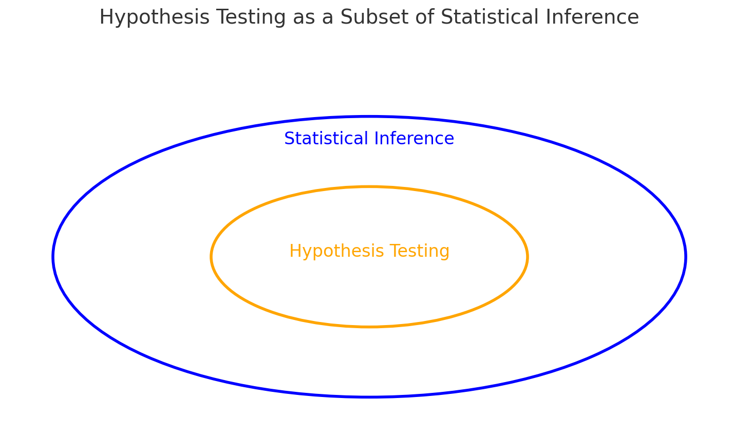
A brief note on hypothesis testing because it often comes up when describing statistical inference. As I hope you realize by now - statistical inference is the big thing. Hypothesis testing is a subset of statistical inference, and quite honestly, it is still hotly debated (even within our profession).

Not long ago this editorial appeared in PTJ:

Mark R Elkins, Rafael Zambelli Pinto, Arianne Verhagen, Monika Grygorowicz, Anne Söderlund, Matthieu Guemann, Antonia Gómez-Conesa, Sarah Blanton, Jean-Michel Brismée, Shabnam Agarwal, Alan Jette, Sven Karstens, Michele Harms, Geert Verheyden, Umer Sheikh, Statistical inference through estimation: recommendations from the International Society of Physiotherapy Journal Editors, Physical Therapy, Volume 102, Issue 6, June 2022, pzac066, https://doi.org/10.1093/ptj/pzac066

This editorial provides recommendations from the International Society of Physiotherapy Journal Editors (ISPJE) addresses the limitations of traditional null hypothesis statistical tests (NHST) in healthcare research, particularly within PT.

Key Points:

Limitations of NHST: NHST involves positing a null hypothesis and calculating a p-value to determine the probability of observing an effect if the null hypothesis is true. However, this method has significant limitations, including misinterpretation of p-values and an overemphasis on statistical significance over clinical relevance.
Estimation Approach: The editorial advocates for an alternative approach known as estimation, which focuses on effect sizes and confidence intervals. This method provides more informative insights by quantifying the magnitude and precision of effects, thereby enhancing the interpretation and applicability of research findings.
Recommendations for Researchers: PT researchers are encouraged to adopt estimation methods in their analyses and reporting. This shift aims to improve the quality and interpretability of research, emphasizing the importance of clinical significance alongside statistical findings.
Editorial Policy Changes: The ISPJE indicates that member journals will expect manuscripts to utilize estimation methods instead of NHST. This policy change underscores the commitment to advancing research practices within the field.

In summary, the editorial calls for a paradigm shift from traditional null hypothesis testing to estimation methods in PT research, promoting a more nuanced and clinically relevant interpretation of statistical data.

Which then created a quick response from a statistician:

Keith Lohse, In Defense of Hypothesis Testing: A Response to the Joint Editorial From the International Society of Physiotherapy Journal Editors on Statistical Inference Through Estimation, Physical Therapy, Volume 102, Issue 11, November 2022, pzac118, https://doi.org/10.1093/ptj/pzac118

In this editorial Lohse addresses the recommendations made by the ISPJE

Key Points:

Critique of ISPJE’s Recommendations: Lohse argues that the ISPJE’s proposal to abandon NHST in favor of estimation methods is premature and may not be universally beneficial. He emphasizes that both NHST and estimation have their respective strengths and limitations, and the choice between them should be context-dependent.
Value of Hypothesis Testing: The editorial defends the utility of NHST, highlighting its role in determining whether observed effects are likely due to chance. Lohse contends that NHST, when applied and interpreted correctly, provides valuable insights, especially in exploratory research phases.
Integration of Methods: Rather than exclusively adopting one method over the other, Lohse advocates for a balanced approach that incorporates both NHST and estimation techniques. He suggests that combining these methods can offer a more comprehensive understanding of research data.
Educational Implications: The editorial underscores the importance of educating researchers on the appropriate application and interpretation of both NHST and estimation methods. Lohse emphasizes that methodological rigor and transparency are crucial, regardless of the statistical approach employed.

In summary, Lohse’s editorial provides a counterargument to the ISPJE’s recommendations, advocating for the continued use of hypothesis testing alongside estimation methods. He emphasizes the need for methodological pluralism and education to enhance the quality and interpretability of research findings in PT.

Connection between statistical inference and hypothesis testing

Now that you understand hypothesis testing (particularly null hypothesis testing - which is the predominant form of hypothesis testing out there) - is controversial, let’s just (for now) connect it to stats inf. This will certainly come up again.

The simplest situation is that you have a sample that includes patients that share something in common, but also have some binary characteristic that separates them. Let’s say they all have a reduced quality of life related to heart failure measured with the Minnesota Living with HF Questionnaire. Some of these patients have characteristic A, other characteristic B. You’re interested in the (alternate) hypothesis that QoL is different (measured using MLHFQ) in people with characteristic A vs. B. Assuming MLHFQ creates quantitative values that are normally distributed in the population we can proceed to test the null hypothesis that they are not different. If we reject the null hypothesis that they are not different, we can state that and then jump to the conclusion that they are different. Notice here please - and this is important - this does not allow me to say that characteristic A vs. B caused the difference in MLHFQ. We’re not there yet.

Why do we think they are different if we reject the null hypothesis? Well, the null hypothesis is the hypothesis that this sample, when divided into two samples (A and B) are from the SAME POPULATION. If they are from the same population, then they are not different and we cannot reject the null hypothesis. What we are trying to say about the divided simples (A and B), is the probability that they are samples drawn from the same population. The probability that they are drawn from the same population is - in essence - the p value. But to get there - we must use statistical inference. We must take the samples and infer population values from them and then consider - based on how much variability there is (and the standard error - meaning how confident we are of the population parameter) - the probability that they are from the same population. By convention - going back to R.A. Fisher in the 1920’s - is that if the probability of the samples being from the same population is less than 5% we should reject that hypothesis (i.e. a p value < 0.05).

With our little example here about MLHFQ scores, if we consider the difference between the two samples (A and B), if they are from the same population the difference in their mean score should be 0. So, we can either run a t-test and get a p value, or we can use the difference as an estimate and calculate a CI. Here’s are some logical inference statements that are bound mathematically:

If p<0.05p < 0.05p<0.05, the confidence interval does not include the null value (e.g., a difference of 0), leading us to reject the null hypothesis.
If p>0.05p > 0.05p>0.05, the CI includes the null value, meaning we fail to reject the null hypothesis.
If p=0.05p = 0.05p=0.05, the CI will just touch the null value (e.g., 0).

This connection shows how both tools—p-values and CIs—ultimately assess the same question: is the observed difference statistically significant?

My more important point - they are all related to statistical inference! :)

Statistical Inference and Population-Level Decision-Making

Statistical inference goes beyond hypothesis testing and confidence intervals—it provides actionable insights that inform decisions at the population level. For policymakers, public health professionals, and researchers, understanding population-wide effects of interventions is crucial for shaping programs and policies aimed at improving health outcomes of a population.

Using Statistical Inference for Policy and Public Health

When statistical analysis reveals that an intervention significantly reduces the risk of a condition—such as heart disease—it allows decision-makers to implement programs with the expectation of similar benefits at the population level. For example:

Risk Reduction in Populations: If a study finds that an intervention reduces the risk of heart disease by 50%, a public health official might roll out a national campaign promoting that intervention, aiming to reduce heart disease prevalence across the country by a comparable amount.
Resource Allocation: Statistical inference can also guide decisions about where resources should be allocated, such as determining which communities might benefit most from specific health interventions.

Population Effects vs. Individual Effects

While statistical inference helps estimate population-wide effects, it does not guarantee the same outcomes for every individual. Many factors influence whether an intervention will benefit a particular person, including:

Individual-level variability (e.g., genetics, lifestyle, socioeconomic status).
Contextual factors that may not have been fully accounted for in the study.

For instance, while the intervention might reduce the average risk of heart disease in a population by 50%, the actual reduction in risk for a given individual could vary widely depending on their unique circumstances.

Key Takeaway

Statistical inference empowers decision-makers to act with confidence at the population level, but applying these insights to individuals requires caution, as the complexity of individual variability often exceeds what can be captured in population studies. Recognizing this distinction is essential for making thoughtful, evidence-informed decisions in both public health and clinical practice.

What is Induction, and How Does It Relate to Inference?

Induction is a reasoning process that moves from specific observations to broader generalizations. For example, observing that a treatment improves mobility in several patients may lead to the generalization that the treatment is effective for most patients with similar conditions. I hope at this point you can see how induction and statistical inference are one and the same. I like to think of induction of the broader larger topic, and statistical inference as a subset of induction in cases were we have enough information to harness the power of probability theory.

Induction provides the framework for us to start to even consider how our statistical inferences can be applied in particular contexts - by considering it’s contrast with deduction.

Deduction starts with general premises or rules and moves to specific conclusions. For instance, if all patients with a condition benefit from a treatment (premise), then a specific patient with that condition will also benefit (conclusion).

Induction (either with or without statistical inference) helps us generate broader generalization that are then taken as general premises that are then used in deduction to develop specific conclusions. This is the start of what I called “dynamic inference” many years ago…. Collins S. Dynamic Inference in Cardiopulmonary PT Practice. Cardiopulmonary Physical Therapy Journal. 2014;25(4). It’s just an abstract from a CSM presentation that never made it to publication. Perhaps this is the year, and perhaps this Substack is the start!

Why Induction & Inference Matter in Clinical Reasoning

Induction is how clinicians learn from experience, drawing broader conclusions from specific patient cases observed over time. However, this process often happens without fully understanding the uncertainty that accompanies these inferences. Clinical research, as experiences with a structured form of observation, uses statistical inference allow induction to quantify this uncertainty. The challenge is that to make research possible - to make those experiences structured - a lot of information is lost. Information that the clinician may find important. There’s a spectrum then - between induction by clinicians, which has the full complexity of clinical situations and statistical inference in research, which limits the full complexity of clinical situation to make the experiences structured.

By integrating research insights, clinicians can enhance their inductive reasoning, making decisions that are both informed by evidence and cognizant of the limitations of generalization.

This is the insight I had in 2005 when I was completing my dissertation and thinking about how to apply what I had learned in all of those epidemiology and biostatistics courses in physical therapy. Admittedly, I also had a growing interest in theology and philosophy which helped fuel the thought process. That insight resulted in the editorial I wrote - and continue to remind people that I wrote :)

Common Challenges and Pitfalls

The fact is that each approach along our spectrum from induction (something all clinicians do if they claim to be learning from their experiences, every time they say “I do X because in my experience,…..Y”) to statistical inference (something all research papers are doing if they claim to be adding knowledge to the profession, every time they say “there is (or is not) a statistically significant effect of X on Y”); there are many biases and fallacies to be considered.

Bias and fallacies will be the topic of an entire page and will be sprinkled here and there - how I teach them here is certainly related to my own biases ;)

Bias and fallacies impact induction (individuals ability to recall and reflect on their experiences); but also impact the experiences themselves (how an experience of a clinician transpires is subject to several biases that impact the experiences themselves, such as confirmation bias). Bias and fallacies impact statistical inference as well - they impact the “internal validity” of structured observations (and are commonly related to how the observations are structured, that is the methods and protocols) and they impact the external validity - the generalizations themselves.

I’m working on a full synthesis of bias and fallacies across the spectrum. While I’m not done yet, I can say this - they are not multiplicative or additive. Meaning, across the spectrum many of the biases and fallacies that are possible cancel each other out and act as guideposts for others when we take a very broad and long look at them in the full synthesis of knowledge based practice. But this requires consideration of the clinicians experience AND the research output.

Critical Realist Lens: A primer

Inductive reasoning, including statistical inference, is essential for exploring causal mechanisms and underlying structures, going beyond surface-level trends to uncover deeper truths. Statistics doesn’t just describe data; it helps us infer how mechanisms and structures interact to produce the observed outcomes.

Grounding this process in Bhaskar’s three domains—empirical (data), actual (mechanisms), and real (structures)—enables more informed and nuanced clinical decisions. For example, while research findings might show a treatment “works” (empirical), a critical realist lens helps us explore why it works by connecting observable effects to deeper causal mechanisms.

This lens also helps clinicians avoid the epistemic fallacy (mistaking observed data for the entirety of reality) and the trap of logical positivism, which overly focuses on surface-level observations. Tools like graphical causal models, which integrate variables across all three domains, are particularly useful in this regard. They allow researchers and clinicians to represent and test relationships visually, making it easier to connect the dots between empirical observations and the mechanisms driving them. By integrating these insights, clinicians can focus not just on “what works,” but also on how and why—ensuring decisions are grounded in a deeper understanding of causality.

Summary & Key Takeaways

Summary of Statistical Inference and Induction

This page explored how statistical inference bridges uncertainty between research and clinical practice, providing a structured way to quantify and navigate the variability inherent in inductive reasoning. Clinicians use induction to generalize from patient experiences, while statistical inference refines these generalizations through tools like confidence intervals and hypothesis testing, but has the consequence of losing some of the fine grained detail of great importance in clinical practice. The integration of research insights with clinical observations, underpinned by a critical realist lens, helps move from “what works” to understanding “why it works” which helps understand how to consider the detailed nuance of particular patient encounters.

Key Takeaways

Statistical inference quantifies uncertainty and supports evidence-informed decision-making.
Inductive reasoning connects evidence to real-world clinical applications.
Critical realism integrates empirical data, mechanisms, and structures for deeper causal insights.

Next Topic

The next page will focus on causality in clinical research, exploring how to move beyond "what works" to uncover the mechanisms, contexts, and conditions behind observed effects including how this might be done in a critical realist review.

A Peripatetic Physical Therapist